This post is 5 years overdue. Fewer and fewer of us train tabular models “by hand” anymore, so the timing could be better, alas. But better late than never.
Background
Back in K Health, we were building diagnostic models for hundreds of diseases and medical conditions. The models’ inputs came from the medical intake we collected, mainly patient demographics and reported symptoms. Each model covered a group of conditions (respiratory, genito-urinary, headaches, and so on), and they were orchestrated like a mixture of experts.
 Image: K Health, via Health Coach Africa
Building each model took months, and every data scientist had their own preprocessing and training scripts living in shadow notebooks. I was tasked with putting an end to this - the goal was an AutoML framework that would let anyone on the team build and deploy a new model in days, not months.
 Image: K Health: Your new primary care doctor?, HBS Digital Initiative
It was the first ML pipeline I’d written for other people to use. Since it had to run without anyone watching, every knob needed a sensible default. For feature selection, none of the standard approaches made sense. The rest of this post presents the solution we opted for, and tries to see, 5 years after the fact, whether it was a good idea.
The standard practice and why it doesn’t default well
Feature selection is almost always done one of two ways. The first is static guessing: keep the top K features, or keep everything above some importance threshold. Either way, someone has to pick the number, whether they hardcode it or try a few values and keep whichever scores best on the validation fold. The second is exhaustive search: run a grid search over K, or use a wrapper like RFECV that fits the model, drops the weakest feature, refits, and repeats until it finds the peak cross-validated score.
Both approaches are suboptimal defaults. A fixed top-K assumes every dataset needs roughly the same number of features, but a simple diagnostic model might need only 5 symptoms while a complex autoimmune model might need 40. Still, hardcoded limits are everywhere, from scikit-learn’s SelectKBest default of k=10 to LightGBM and XGBoost pipelines where teams habitually keep the top 20 or 50 features. To see how practitioners actually set this knob, I scanned one million public Kaggle notebooks and Python scripts. Two thirds of the explicit choices are a round number:
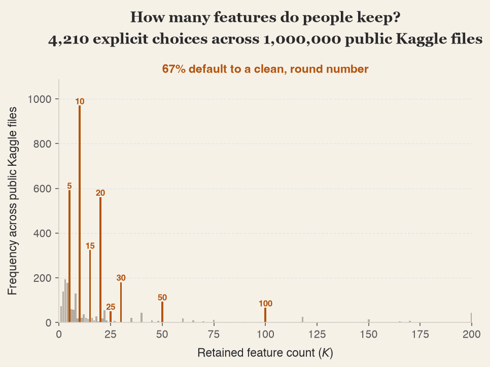
A static threshold (like importance > 0.01) is just as brittle. It assumes an importance score means the same thing regardless of how many features there are. But impurity-based importances (scikit-learn’s .feature_importances_) are normalized to sum to 1 across all columns, so a score is relative, not absolute: add more columns and each one’s share shrinks.
An exhaustive search like RFECV solves the adaptability problem by brute force, refitting the model dozens or hundreds of times per run. That’s fine for a single model, but in a pipeline that trains many models and retrains them on a schedule, it becomes the most expensive step. So the requirement was clear: something that adapts to the data like a search, without paying for one.
The solution: borrow the PCA trick
If the optimal number of features is a property of the dataset, the principled approach is to estimate it directly rather than guess an integer or brute-force a search. We can’t derive that number in advance, so we need a proxy for it.
We already have feature importance scores; we just need to trust them to rank the columns by predictive power. Once the features are sorted, the only remaining question is when to stop.
The idea, borrowed from PCA, is to stop by cumulative sum. Just as PCA(n_components=0.95) keeps 95% of the variance without hardcoding a component count, we do the same for raw features: sort by importance, walk down the running sum, and cut once we reach 95% of the total. We’ll call this preserved importance.
The premise is that a relative target like “keep 95% of the importance” transfers across datasets better than rigid rules like “keep 20 features” or “keep everything above 0.01.”
Preserved importance, precisely
To be mathy about it: denote the normalized importances, sorted from largest to smallest, as . We keep the smallest number of top features whose importance reaches the target :
In code it’s about 10 lines:
import numpy as np

def cumulative_mask(importances: np.ndarray, theta: float = 0.95) -> np.ndarray:
    """Boolean mask for the fewest top features whose importance sums to >= theta."""
    importances = np.clip(importances, 0, None)  # Permutation importance can go negative
    total = importances.sum()
    if total == 0:
        return np.ones_like(importances, dtype=bool)  # No signal anywhere; keep everything

    normalized = importances / total
    order = np.argsort(normalized)[::-1]
    cutoff = np.searchsorted(np.cumsum(normalized[order]), theta) + 1

    mask = np.zeros_like(importances, dtype=bool)
    mask[order[:cutoff]] = True
    return mask
In practice
In theory, it makes sense. But in theory there’s no difference between theory and practice…so let’s run an experiment.
I used three datasets: Breast Cancer (30 features), MNIST (784 pixel features, subsampled to 8,000 of its 70,000 images to keep the runtime reasonable) and Isolet (617 speech-signal features, 26 classes). In the last two the signal is spread across hundreds of columns, which is where a fixed K should struggle. For each dataset, I rank features by Random Forest importance and compare three selection rules against using all features: Top-20, a >1% threshold, and Cumulative-95. Accuracy is averaged over 10-fold cross-validation.
| Dataset | Top-20 | Static (>1%) | Cumulative-95 | All features |
|---|---|---|---|---|
| Breast Cancer | 0.965 | 0.960 | 0.963 | 0.963 |
| MNIST | 0.776 | 0.228 | 0.944 | 0.943 |
| Isolet | 0.797 | 0.133 | 0.949 | 0.946 |
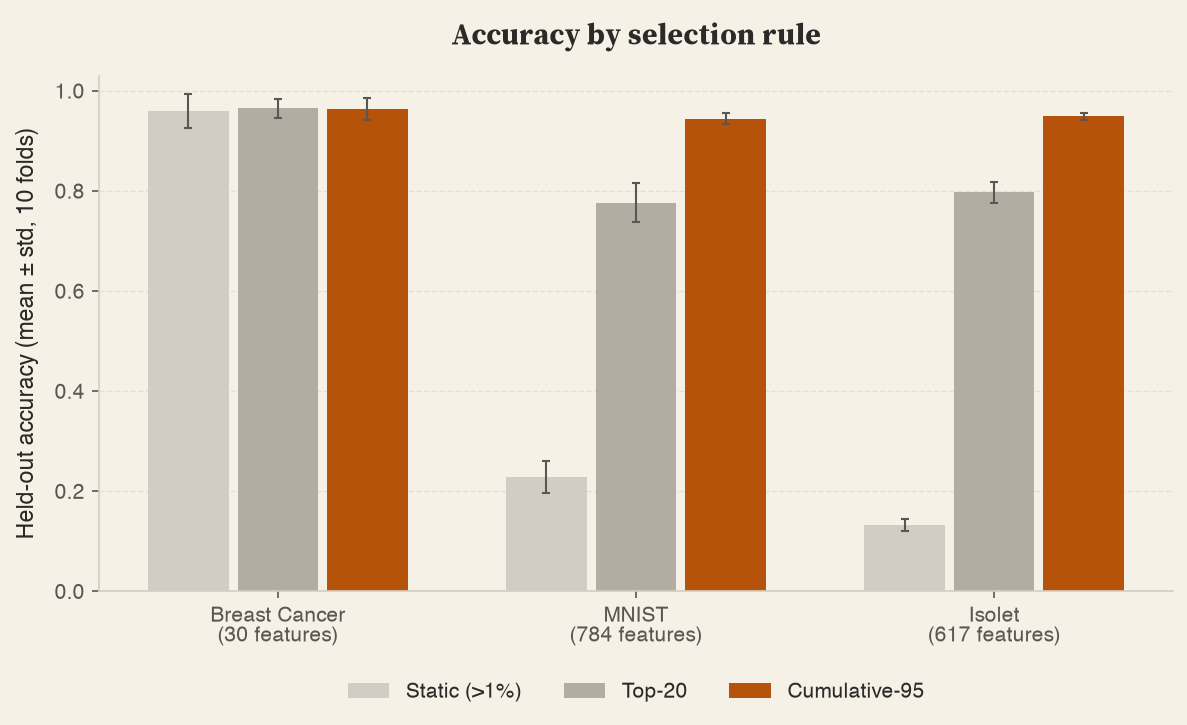
On Breast Cancer, Cumulative-95 keeps about 20 features, the same as Top-20, and the three rules tie within noise. On MNIST and Isolet it keeps 324 and 496 features and matches the full-feature accuracy, while Top-20 trails by 17 and 15 points.
The static threshold keeps a single feature on MNIST and Isolet. With importance spread over hundreds of columns, almost no feature exceeds 1%, and accuracy falls to 0.23 and 0.13.
Parting thoughts
One experiment does not convince of anything. But I hope it demonstrates the potential of what a few lines of code, that have no compute downside, can give. From my experience, this has proved to work very well. Give it a try!
Addendum
All this talk about adapting to data reminded me of this very interesting read by Joshua Fost, which claims that what we really want in life is adaptive complexity.